
We continue our series about the Kalman filter based on the example of Roger Rabbit. Please refer to the Intuitive introduction to the scalar Kalman filter page, where we develop the Roger Rabbit experiments.
1. Roger Rabbit does not obey the constant movement model
You are so happy that you increased your
chances to hit the animal. But Roger is excessively smart. It now runs
along the line, while changing its speed and its direction. Your simple
model ![]() has
become absolutely useless. So, you choose to ignore the model and come
back to the temporary supposition that Roger's position does not change
and you want the Kalman filter to follow the measurements alone.
has
become absolutely useless. So, you choose to ignore the model and come
back to the temporary supposition that Roger's position does not change
and you want the Kalman filter to follow the measurements alone.
Perhaps the reader already noticed that when we were talking about "ignoring the model", this was not an exact formulation, because, in fact, the Kalman filter was told to consider Roger's position to be invariable. It must be underlined that the "invariability" also represents a model with speed being constantly zeroed. At first glance telling the Kalman filter that the variance is 0.55 doesn't make much sense. However, if the filter is configured that way, it will not completely trust the constant model and allow the state estimations to be adapted according to the measurements. Curiously the estimation is not that bad as shown on the graph of paragraph 3 of the Intuitive introduction to the scalar Kalman filter page.
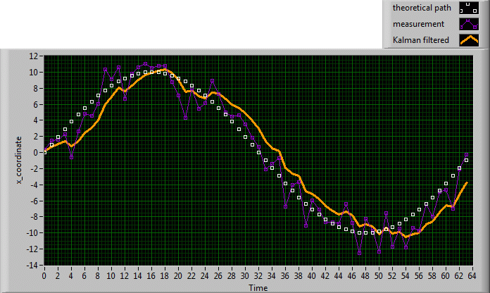
We now suppose that Roger Rabbit runs forth and back, obeying a sinusoidal 1D path. Our measurements still have variance R=4. Under these conditions the result can be compared to a smoothed FIR-filtered signal that lags the original measurement signal (Fig. 1). The Kalman filter has lost all its power of prediction, because at any moment it returns the estimation of an earlier state, as the a posteriori estimation changes only through the effects of the residual that is calculated later than the bad a priori estimate. Again the arising question, whether we can improve this, may be answered: Yes, we can!

Fig. 1 : If the Kalman filter assumes a constant model, it looses its prediction power.
2. Estimating Roger's speed
So far our a priori estimation
equation has been ![]() ,
in this case with s=0. But, since we are estimating Roger's position rather well,
nothing prevents us from using the positioning for the a priori estimation of
Roger's actual speed.
,
in this case with s=0. But, since we are estimating Roger's position rather well,
nothing prevents us from using the positioning for the a priori estimation of
Roger's actual speed.
So, we admit (with ![]() ):
):
![]()
We cannot improve this a priori estimation through an a posteriori speed estimation, because we have no direct measurement of Roger's velocity. But, if we feed this speed estimation into the a priori path estimation equation, we get:
![]()
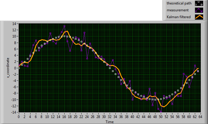
Note that these equations vaguely contradict the Markov process postulate, for the simple reason that we go back into the past more than one time step. Here we are no longer in the theoretical foundations of the Kalman filter, but in the very practical application of the algorithm. The result is amazing, because the time-lag disappears, as can be seen on (Fig. 2).

Fig. 2 : If the Kalman filter uses the described a priori speed estimation, the time lag disappears.
3. Adding the second observer
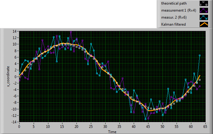
If now we add the second observer, who measures with a poorer variance R2=6, the state estimation is drastically improved (cf. Fig. 3). Summarized we can say that with the scalar Kalman filter, we are able to rather precisely estimate Roger Rabbit's position, even if we have no direct estimation or measurement of the rabbit's speed.

Fig. 3 : The second observer data dramatically improves the path estimation. Roger's fate is sealed.