
Imagine that you are hunting Roger Rabbit. Once again you are lying in wait for that beast, because it narrowly escaped a few times and you definitely want to shoot it. You have hidden at 200m with your rifle scope screwed to your best hunting shotgun... and you are waiting. You are aware that your accuracy at that distance is 50cm, so you must be certain of your shot... and Roger is clever and overly swift. You estimate its running speed at about 1.50m per seconds, quite impressive for a rabbit, isn't it? Your bullet is flying at 800m/sec.
You catch sight of the rabbit. It scampers in the free field. Excellent conditions; you rapidly calculate that you must target a point, 37.5cm ahead of Roger's actual position. Bang !... and you missed it. What went wrong?
Because your cockily neighbor always returns triumphantly from hunting and you have failed so often, you are questioning yourself, if there is a way to improve your estimation of Roger Rabbit's position, so that you can hit that bunny. The answer to that question is yes, you can! If you are able to correct your prediction with your best observation, then you will reduce the errors to a minimum. That's exactly what the Kalman filter is for!
First let's observe Roger's exact path along the 1D-line. Suppose that we do this with the help of an error-free laser system. The measurements are taken regularly each second.
1. Modelling Roger Rabbit's path
We call Roger's
exact position the
state of the system: x
. We expect that the rabbit is running at constant
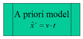
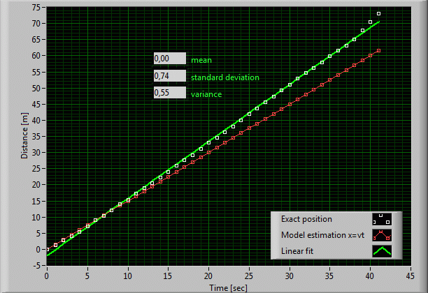
speed and that the position is given by the simple equation ![]() .
However we must conclude from the function graph that the speed isn't
exactly constant. Because the equation only is an approximate description
of the state that is effectuated BEFORE doing anything else, the symbol
"x"
is marked by a caret, standing for the estimation, followed by the
superscript minus, which stands for the timing "before" or
" a priori". Our postulated function underestimates Roger's
real speed. That's real life: Roger isn't running along a clean line,
because it has no possibility to verify and maintain its speed at a
constant level on a terrain that is rough and slippery. If we use the statistical method of the linear
fit, we draw a line of the ideal path that would guarantee a
constant speed. This line is a bit steeper than our initial prediction.
The linear fit method has the particularity of minimizing the sum of all
the deviations from the ideal line. To be precise, it minimizes the sum of
the squared errors. The mean of the absolute errors obviously is zero,
because positive and negative errors annihilate each other. The standard
deviation is 0.74[m]. (Note that the variance is the square of the
standard deviation). The standard deviation is an indicator of how far the
data points spread around the ideal line. We denote Q=0.55
the variance of the state noise. (In the case of Roger Rabbit, we assume
that from many earlier observations, we have been able to deduce this
estimation of the variance, because by no means we are able to directly
measure the noise.)
.
However we must conclude from the function graph that the speed isn't
exactly constant. Because the equation only is an approximate description
of the state that is effectuated BEFORE doing anything else, the symbol
"x"
is marked by a caret, standing for the estimation, followed by the
superscript minus, which stands for the timing "before" or
" a priori". Our postulated function underestimates Roger's
real speed. That's real life: Roger isn't running along a clean line,
because it has no possibility to verify and maintain its speed at a
constant level on a terrain that is rough and slippery. If we use the statistical method of the linear
fit, we draw a line of the ideal path that would guarantee a
constant speed. This line is a bit steeper than our initial prediction.
The linear fit method has the particularity of minimizing the sum of all
the deviations from the ideal line. To be precise, it minimizes the sum of
the squared errors. The mean of the absolute errors obviously is zero,
because positive and negative errors annihilate each other. The standard
deviation is 0.74[m]. (Note that the variance is the square of the
standard deviation). The standard deviation is an indicator of how far the
data points spread around the ideal line. We denote Q=0.55
the variance of the state noise. (In the case of Roger Rabbit, we assume
that from many earlier observations, we have been able to deduce this
estimation of the variance, because by no means we are able to directly
measure the noise.)
2. Measuring Roger's path
Now it is certain that we are not capable of measuring Roger's position as exactly as assumed before. This means that we are not able of observing the system state directly. It's common that measurements are error-prone, so let's suppose that our measurements z are noisy with variance R=4.
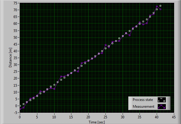
This graph shows that we are measuring something quite different from reality, although the values also spread around the rabbit's path. If we rely on the measurements alone, the probability of missing Roger therefore is very high. The measurement signal -as a real data train- now carries along information about the state that has been injected with noise from Roger's non-constant movement and from the unsatisfying quality of the measurements. Both noise sources are uncorrelated, which means that the state noise does not bias the measurement noise and vice-versa. The main question is, whether it is possible to detect the state behind the clouds of noise. And again, we may affirm: Yes, we can ! With the Kalman filter !
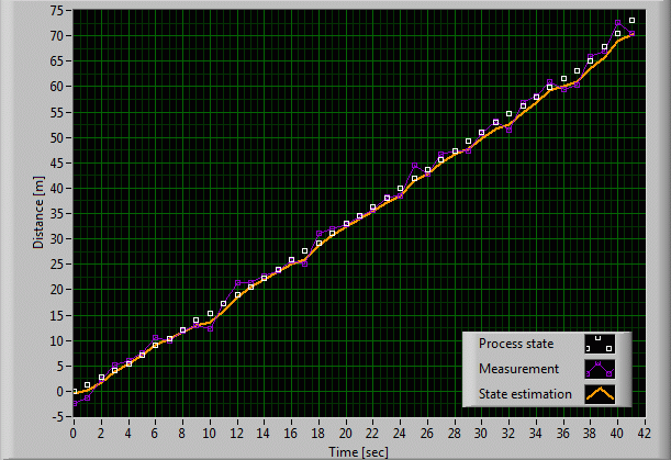
3. Estimating Roger's path with a Kalman filter ignoring the model
Let's plunge into the
Kalman filter functionality without analyzing anything of its internals! The following graph
shows a first Kalman filter estimation of Roger Rabbit's path that takes
into account your measurements. For the
moment it starts
from the (wrong) assumption that the state is constant and Roger is not
moving. Nonetheless the filter process does not completely trust
this very bad state model, accepting a state noise variance of 0.55. It
doesn't blindly believe the measurements either, because it takes into
account the measurement noise variance of 4. Therefore the filter delivers a growing state estimation
that contradicts the bad temporary assumption of Roger's immobility. Since
the estimation is the result of your observation, it is called the a
posteriori estimation and is symbolized with ![]() .
.
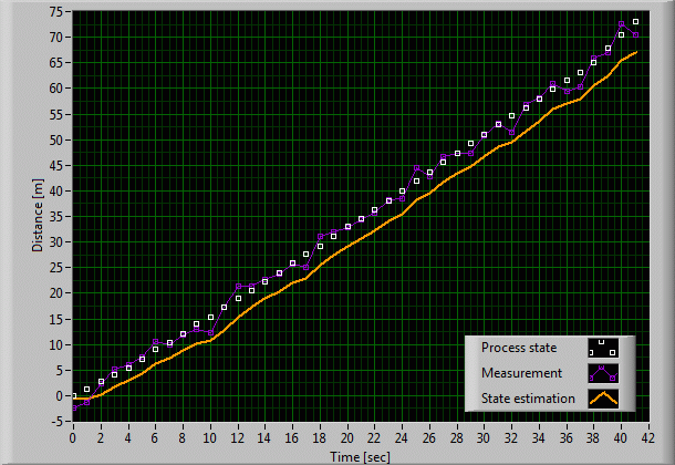
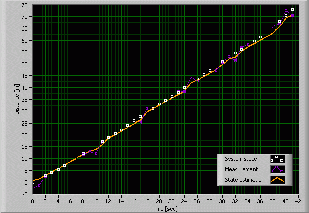
4. Estimating Roger's path with a Kalman filter including the model
We can improve the
filter response by telling it that we did not suppose the state to be constant. We know that Roger is running, so we inform the Kalman filter
that according to our best knowledge of the bunny, it will behave
according to the deterministic model ![]() . (Again, at the moment, we do
this without venturing forward into the mathematical machinery of the
Kalman filter.) The result is simply amazing, as can be seen on the next
graph. There still is a slight drift from the true state, but Roger's
estimated path is within your shooting accuracy during most of the time.
Roger should start praying! Note that the Kalman filter can easily be
tuned through a few useful parameters, in order to improve the output.
. (Again, at the moment, we do
this without venturing forward into the mathematical machinery of the
Kalman filter.) The result is simply amazing, as can be seen on the next
graph. There still is a slight drift from the true state, but Roger's
estimated path is within your shooting accuracy during most of the time.
Roger should start praying! Note that the Kalman filter can easily be
tuned through a few useful parameters, in order to improve the output.
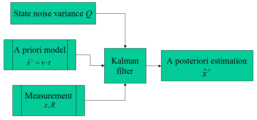
One of the great features of the Kalman filter is
the fact that
through the deterministic model, you get a prediction
of the next state of the system. Thus from the last best state estimation you will be able to forecast Roger's next position by
applying an approximate system description. Anyway, because your shot
takes so long, you need to anticipate where Roger will be in some near
future. So, you base your guess on the best knowledge of the system, its statistics and
naturally of your faculty of observation. During the prediction step, the
Kalman filter also guesses the quality of the prediction in the form of
the a priori variance of the process noise denoted ![]() , where the
latter is defined as
the error between the true state and the a priori state estimation. In the
next step the filter then proceeds to the correction
of the state forecast on the base of the measurement. Since it is the all over goal of
the filter to minimize the process error, the correction will also be
applied to the error estimate. The result is the a posteriori process
noise variance
, where the
latter is defined as
the error between the true state and the a priori state estimation. In the
next step the filter then proceeds to the correction
of the state forecast on the base of the measurement. Since it is the all over goal of
the filter to minimize the process error, the correction will also be
applied to the error estimate. The result is the a posteriori process
noise variance ![]() .
.
5. Estimating Roger's path with a Kalman filter ignoring the model under the condition of incomplete measurement data
Let's suppose that Roger Rabbit is really clever and prefers a path along the border of a copse. You will have serious difficulties in distinguishing the rabbit from the background, if it passes trees with barks that have almost the same colour as its own fur. At those moments you cannot trust your observation and the measurement noise variance grows significantly. If Roger reappears between the trees however, you will be able to localize it again with the same accuracy as before.
6. Estimating Roger's path with a Kalman filter including the model under the condition of incomplete measurement data
Now we alter the experiment by re-adding the
initial model ![]() to the filter. The observation noise variance obeys to the description of experiment 5. Now the Kalman filter starts trusting the
improved model
during the non-valuable measurement phases. The result is amazingly
accurate, despite the bad observation. With the Kalman filter, Roger Rabbit's
chances have seriously aggravated.
to the filter. The observation noise variance obeys to the description of experiment 5. Now the Kalman filter starts trusting the
improved model
during the non-valuable measurement phases. The result is amazingly
accurate, despite the bad observation. With the Kalman filter, Roger Rabbit's
chances have seriously aggravated.
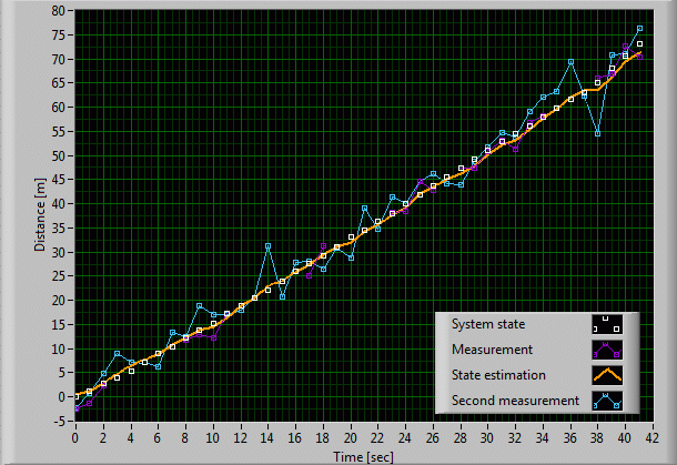
7. Adding a second observer
Roger tried to finesse you by disappearing in the background. Your Kalman filter helped you to rival the rabbit. But, you want to get almost certainty of shooting that bunny in order to avoid the mockery of your unsympathetic neighbor. So, this time you ask a friend to help you. Four eyes are more than two. You post him to a strategic place on a hill, where he can observe everything well and share his measurements with you. Because he is further afar, the noise variance of his measurements is set to R2=16. The Kalman filter fuses your friend's measurement with yours. The additional information reduces the process noise and this time, except for the very end phase, Roger's fate should be sealed.
8. Conclusion
With the help of the Kalman filter, Roger Rabbit's path can be estimated accurately. The method unlocks enough information from the initial deterministic model that is merged with uncertain and noisy measurements.