Binaural sensor
(how to localize the origin of a music signal or a human voice)
last update 8/3/2003
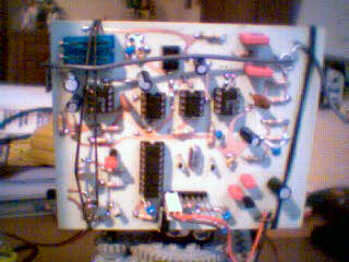
This brand new sensor prototype still is at experimental stage for the one only reason, that the dimensions of the PCboard are too large. But the sensor perfectly works as you can see on the video:
Click to see the video (940kB)
Amateurs of our web-site have already studied our different sound localizing sensors. There have been two classes of sensors:
The first class allows the localizing of a continuous sound-source, in the case of two (or even more) well-calibrated sensors separated by a shadow-producing object. A potential robot-brain, for example, can decide whether to walk to the right or to the left, depending on the the signal-strength detected at each microphone. The major disadvantage is that the robot may go wrong because of echoe-signals. Echoes even could entirely corrupt the result. Another problem with this kind of sensors is the fact that level differences only appear at frequencies above 500Hz.
The second class gives the possibility to prune those echoes in a very simple way. In the case of an echo, the duration of flight becomes greater than the maximal time given by the distance between the microphones. The problem of this approach is that the sound-wave has to be identified clearly. Normally this is done through a peak detector. When the peak passes a certain threshold at microphone 1, the brain starts time-measuring and waits for the impacts at the microphones 2, 3.... Such a sensor may only react on loud pulses such as clapping, finger snipping, screaming a.s.o. Continuous reading of sound-signals is not possible.
1. Continuously determine the Interaural Time Difference (ITD)
The sensor presented here belongs to a third class. Through a mathematical procedure known as cross-correlation the sensor yields the difference of phase of the signals. Because the microphones are located at different places, the sound-wave arrives with certain delays at the implied microphones. If, in the case of two microphones, the phase is zero, the sound source is located on the mediatrice of the segment [Mic1, Mic2]. If there is a difference of phase, the delay will not be measured directly, but computed from the signals. This may be done with analog or digital means. We opted for a digital solution.
The signals are out of phase on this picture.
There exist various ways to compute the cross-correlation. We followed our standard route: "Do things simply!" As we have to deal with a real time problem, computation speed plays an important role here.
Preliminary note: the present device is a two channel sensor. Let's suppose both signals in phase. The Lissjou-graph, which may be easily obtained with an oscilloscope by leading one channel to the vertical and the other to the horizontal input, shows a straight line. If both signals have the same amplitude, the line's slope is 45°. Out of phase, the graph takes complex forms. If a Linear Fit is operated to the data, in our example, we obtain a Mean Square Error (MSE) of 5.76 .
If - in phase - the amplitudes don't match exactly, the slope of the line changes. Adding some random data, causes a slight transform of the aspect with MSE still small around 0.54 .
The way to yield the difference of phase roughly is to overlay both signals while processing additional phase deviations and choose the one which produced the minimal MSE.
The heart of our device is a microcontroller which reads a certain number of data on two A/D-channels. The sampling of the audio signal is operated at 30kHz. The program scans and compares a signal sub-set from the right channel with the datasets from the left channel. If there is a match, the offset-index is proportional to the phase.
Problems may appear at regular shaped signals above 1500 Hz. In these cases there will actually appear two (or even more) matching indexes. But this will not happen with human speech or any other composite signals, even if faster than 3000 Hz. For instance, white noise is always localized.
Echoes are pruned at source through this procedure, because no comparison is operated for phases greater than the maximum given by the microphone distance. However, standing waves, generated through room-resonances -especially at low frequencies - may corrupt the result.
Block-diagram:
The micro-controller program has the following aspect:
The whole process is repeated at about 400 Hz. The update of the output-voltage is done at 40 Hz. The result is a voltage which is proportional to the direction of the sound-source (-90°,90°).
2. Where is the beef?
Mathematical analysis of the sound direction:
From our sensor we get a value which is proportional to the phase-deviation between the left and right signals. This value has a dimension of time. Multiplied with the sound-velocity changes the dimension to distance.
Let's call the output d, and a = | d / 2 |
The microphones shall be located at F(-c,0) and F'(c,0)
Let's determine all the points M(x,y) that :
example:
c = 5 [cm], dt = 0.1ms ==> dx = 3.43 cm, the sound-velocity being 343 m/s
==> a = 1.715 ; a2 = 2.9412 ; b2 = 25 - 2.9412 ; b = 4.7
As we can see on the picture, for any sound source located at more than 10 cm from the microphone, the slope of the asymptotes gives a highly accurate direction. To have an additional directional information about rear and front, we choose microphones with high directional caracteristics. By this way, signals from the rear are not considered, the rear half-plane can be eliminated as origin of the sound source.
Thus the slope is given by:
The following representation shows that our more intuitive formula from the former projects is a very good approximation of the direction, expressed as a linear equation: y = ux + v. There is only an unprecision if the sound-waves arrive parallel to the microphone-axes.
3. Testing the device
We explained above that we are taking 30 samples. To be precise, the microcontroller actually takes 36 samples. Thus there are 25 sub-datasets which are considered in the cross-correlation computation. Therefore the maximum expected device precision is 180° / 25 = 7.2° .
The following Robolab-test gives us a standard deviation of 15.9° which is twice our expected value.
The next diagram shows all the measured data-points M(raw,angle), where raw means raw-sensor value and where angle corresponds to the azimuth in degrees read by the rotation sensor.
The following diagram shows the deviation from the real angle of the computed angle in function of the sensor-data .
4. Schematics
The electronics circuit is made of 5 parts:
The voltage regulator is known from several of our pages, so does the low-pass filter which is connected to the PIC-PWM-output of the PIC, and also the IR-device. (Have a look at former advanced sensor projects http://www.convict.lu/Jeunes/RoboticsIntro.htm )
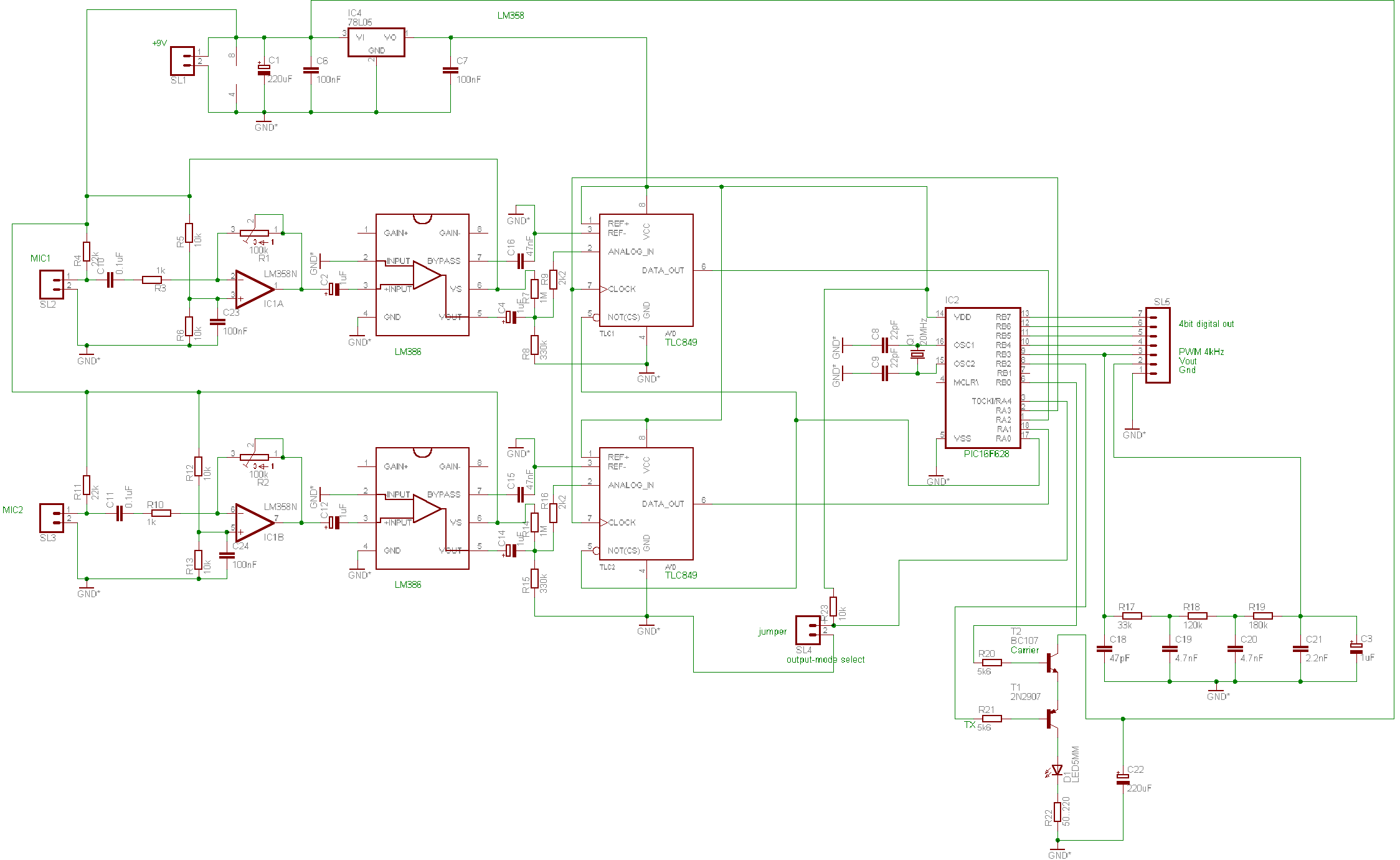
Let's have a closer look to one of both signal channels :
A first amplifier stage allows a clean amplification of the weak signals arriving from the microphone. C23 (100nF) helps decoupling the stage from the rest of the circuit, especially from the 30kHz clock signal generated by the PIC to clock the TLC849.
The second stage is made with the well-known audio-amplifier LM386. Pin 1 and 8 are not connected. This configuration provides a gain factor 20. The output-signal of this stage is biased to a center-voltage of 2.5V through the divisor R7 / R8. The 8-bit A/D converter TLC849 was chosen for two reasons:
This allows a nearly synchronous conversion of the two signals at 30kHz (chip-select, clock, data-transfer and storage into PIC-memory).
5. PIC program
The TLC849 is an easy to manipulate chip. Its datasheet explains that the conversion cycle, which requires 36 internal system clock periods (17microseconds maximum), is initiated with eight I/O clock pulses trailing after CS goes low. The 8 clock pulses are also used for the serial transmission of the previous conversion data.
Note that the program operates the first conversion to activate both TLC849s correctly. For every successive iteration, the last converted value is indirectly stored. The pointers are incremented. The data-transfer is done through eight clock pulses. Buffers are shifted one digit. Again we present the program in the easy to understand quasi-Robolab flowchart-form.
We'd like to keep the tricky cross-correlation-procedure hidden. Note that together with minimizing and PWM-output, it takes 1ms to proceed all the necessary computations.
Here the PWM-output sequence:
For anyone who is interested in the ready programmed micro-controller, please contact the web-master.
6. Resources