A simple and fast look-up table method to compute the exp(x) and ln(x) functions
Claude
Baumann, Director of the Boarding School „Convict Episcopal de Luxembourg[i]“,
5 avenue Marie-Thérèse, m.b. 913, L-2019 Luxembourg[ii]
claude.baumann@education.lu
July 29th
2004
Abstract
Normally
today’s computers shouldn’t present any problems to rapidly calculate
trigonometric or transcendental functions by any means. Developing better
algorithms appears to be more sporty than really practical. However the growing
number of embedded applications based on micro-controllers may ask for gain in
speed and memory economy, since those applications are fundamentally
characterized by limited resources and optimized designs in order to reduce
costs. Thus, fast and memory economic algorithms keep playing an important role
in this domain.
The present
algorithm was developed during the elaboration of Ultimate ROBOLAB, an
extension to the ROBOLAB software[iii]
, known as a powerful graphical programming environment for the LEGO RCX. By
difference to standard ROBOLAB that works with interpreted code, Ultimate
ROBOLAB[iv]
directly generates Assembly code from the graphical code, compiles it to
Hitachi H8 byte codes which are then downloaded to the RCX.
The
algorithm has three important sections: the first one -universally known-
consists in reducing the function f(x)=exp(x) to f0(x)=2x
- respectively g(x)=ln(x) to g0(x)=log2(x) - the second
section concerns the arrangement of the numbers in the particular way to have
the CPU only compute f0(x) or g0(x) for x Î [1,2[ and the third manages a fast computing
of f0(x) and g0(x) to any desired precision according to
a look-up table composed of 22 numbers only for IEEE 754 standard single
precision floating point numbers. During the execution of the elementary
functions, in any case the CPU has to operate less than 22 products. The
average case turns around 11 multiplications.
Introduction
The
development of Ultimate ROBOLAB, a LabVIEW-based graphical compiler for
Hitachi H8/300 code, is a particularly interesting demonstration of the typical
constraints to which embedded design with micro-controllers may be submitted. Ultimate
ROBOLAB is destined as a development tool for advanced users of the
well-known LEGO RCX. This module had been invented as the central part of the
LEGO Robotics Invention System (RIS), a highly sophisticated toy that, due to
its excellent features, has found many applications as an educational tool in
schools, high schools and even universities.
The heart
of the RCX is a 16MHz clocked Hitachi H8/3292 micro-controller. Besides
peripheral devices and 16kB on-chip ROM and 512 bytes RAM, this
micro-controller encapsulates an H8/300 CPU that has eight 16-bit registers
r0..r7 or sixteen 8-bit registers r0H, r0L, … r7H, r7L (r7 is used as the
stack-pointer); 16-bit program counter; 8-bit condition code register;
register-register arithmetic and logic operations, of which 8 or 16-bit
add/subtract (125ns at 16MHz), 8.8-bit
multiplying (875ns), 16¸8-bit division (875ns); concise instruction
set (lengths 2 or 4 bytes); 9 different addressing modes. Together with 32k
external RAM, LCD-display, buttons, infrared communication module, analog
sensor ports and H-bridge output ports, the RCX is an ideal instrument for the
exploration of micro-controllers in educational contexts.
In order to
attribute most flexibility to the RCX for all kind of robot projects, the
programming environment Ultimate ROBOLAB required a firmware kernel that
should guarantee memory economy and execution speed. Thus each part of the
kernel had to be optimized to the limits, so that users could dispose of a
maximum of memory for their own code and sufficient reaction speed for reliable
robot behaviors and closed loop controls. This was particularly challenging concerning
the inclusion of an advanced mathematical kernel that comprised IEEE 754
standard single precision floating-point operations, among which the square
root, trigonometric and exponential functions. Scrutinizing the subject with
the target to find algorithms that could best balance the requirements rapidly
ended in the choice of Heron’s algorithm for the square root and CORDIC[v]
for the trigonometric functions. However the exponential functions revealed
themselves as more difficult.
1.
Different methods of calculating y=exp(x) and y=ln(x)
In order to
dispose of valuable algorithms for the exponential function and its reciprocal,
several existing methods have been evaluated. An alternative CORDIC[vi]
algorithm using a hyperbolic atanh table instead of the atan
value list was the first possibility that we tested applying the equations:
But the
implementation of this solution led to an excessively long and complex code, because
of a necessary additional algorithm to assure the convergence. Another
alternative was an application of Taylor’s series:
While being
easily programmable, these series present the disadvantage of converging only very
slowly, leading either to unacceptably long computing time or unsatisfying
inaccuracy.
Other
high-speed alternatives known from FPGA or DSP implementations, and based on
large constant tables had to be excluded as well. A remarkable representative
of efficient table based algorithms was presented by DEFOUR et al[vii],
who succeeded in obtaining high precision function approximation with a
multipartite method by performing 2 multiplications and adding 6 terms. The
trade-off, and the reason for the disqualification in our application, is that
the table size grows exponentially with the precision. For example, in order to
get 23 correct bits, corresponding to an error of ½ ulp (units in
the last place) in the case of IEEE 754 standard single precision
floating-point data, the exp(x) function needs a table size of 82432 constants.
Obviously such a table would explode the RCX memory capacity.
A better
approximation choice was the use of a polynomial series based on error
minimizing Chebycheff[viii]
nodes[ix].
For the purpose of y=2x, xÎ[1,2[ , the applied function to
determine 10 Chebycheff-points is:
![]()
These nodes
serve as reference-points for a 9th order polynomial curve fitting.
While applying the Horner Scheme[x]
to the polynomial, the number of operations is a total of 9 multiplications and
9 additions per function call, compared to 7.2 + 1=15 multiplications and 9 additions for the
straightforward polynomial calculation.
The
accuracy that can be obtained with the algorithm is about 3E-7, as can be seen
in the result of a LabVIEW simulation (picture 2).
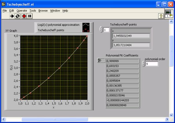
Picture 1: Operating the polynomial fit with
LabVIEW 7.1 on the base of 10 Chebycheff nodes.
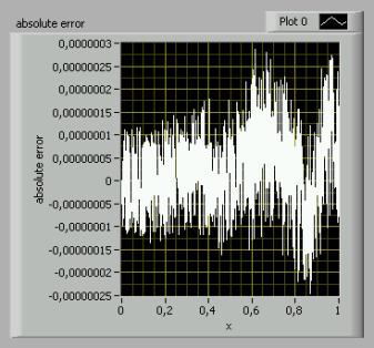
Picture 2: Absolute error of the previous polynomial
approximation. (mse=0.33)
A similarly
efficient polynomial approximation could be set up for the log2(x)
function in the special case of xÎ[1,2[ . Of course satisfying
algorithms must be added to extend the functions to the ranges ]-¥,+¥[ respectively ]0,+¥[ .
The further
investigation of the subject however led us to the algorithm that is described
in this paper as a better solution for the purpose, combining memory economy
and execution speed in the case of IEEE 754 standard single point precision
floating-point representation[xi].
2.
Calculation of f(x)=exp(x)
2.1.
Simplification to f0(x)=2x
For any
real x we have:
This
equation signifies that any x must be multiplied with the constant c=1/ln(2)
before computing the f0 function.
Convention:
we may suppose x>0, because of the trivial e0 =1 and e-x
= 1/ex allowing an easy computation for any x.
2.2.
Arranging of f0(x)=2x
The IEEE
standard floating point representation transports three information-parts about
the concerned number: the sign, the biased exponent and the fractional part
(=mantissa).
Example: single precision representation
00 01 02 03 04 05 06 07 08 09 10 11 12 13 14 15 16 17 18
19 20 21 22 23 24 25 26 27 28 29 30 31
s e e
e e e e e
e m m m m
m m m m m m m m m
m m m m m
m m m m m
where :
Ø
if e=255 and m<>0, then x = NaN (“Not a
number”)
Ø
if
e=255 and m=0, then x = (-1) s * ¥
Ø
if
0<e<255 then x = (-1)s*2(e-127) *
(1.m) with (1.m) representing the
binary number created by preceding m with a leading 1 and the binary point
Ø
if e=0
and m<>0, then x = (-1)s*2(-126) *
(0.m) representing denormalized values
Ø
if e=0
and m=0 and s=1, then x = -0
Ø
if e=0
and m=0 and s=0, then x = 0
The
particular representation of the number 2.25 therefore is:
1.
s = 0
2.
e = 1 +
127 = 128 = b’10000000’
3.
m =
0.125 = b’0010000 00000000 00000000’
Normalized
mantissas always describe numbers belonging to the interval [1,2[ .
Convention:
unbiased exponent = q (integer)
x = (-1)s*2q
* (1.m)
Note: it is
not possible to represent the number 0 in this form!
2.3
Study of f1(x = 1.m) = 21.m
![]()
![]()
(formula
1)
In any case
we have: 2(x-1) Î[1,2[, since  or simpler:
mÎ [0,1[ Þ 2mÎ[1,2[
Thus the
result 2(x-1) will always be normalized to the IEEE standard.
To fast
compute 2(x-1), we only need to first set up a look-up table with the
constant values of successive square-roots of 2, then operate consecutive
multiplying of a selection of those numbers while scanning the mantissa m of x.
The table is filled with values that have been previously yielded by any
iterative means with a precision <0.5 ulp. (For instance in a
practical micro-controller application, the values can be produced by the
cross-compiler host and stored as constants in the micro-controllers ROM,
EEPROM or even as part of the program-code). Due to the limitation of accuracy
of the single precision representation, the LUT only needs 22 different values.
Thus the last bit won’t add any information as can be seen in the following
example. (For better comprehension, we added the value 2 to the table at index
0.)
Example:
Compute y = 21.171875
Look-up
table (LUT):
|
index |
|
|
0 |
2 |
|
1 |
1.41421353816986084 |
|
2 |
1.18920707702636719 |
|
3 |
1.09050774574279785 |
|
4 |
1.0442737340927124 |
|
5 |
1.02189719676971436 |
|
6 |
1.010889176330566 |
|
7 |
1.00542986392974853 |
|
8 |
1.00271129608154297 |
|
9 |
1.00135469436645508 |
|
10 |
1.00067710876464844 |
|
11 |
1.00033855438232422 |
|
12 |
1.00016927719116211 |
|
13 |
1.00008463859558105 |
|
14 |
1.00004231929779053 |
|
15 |
1.00002110004425049 |
|
16 |
1.00001060962677002 |
|
17 |
1.00000524520874023 |
|
18 |
1.00000262260437012 |
|
19 |
1.00000131130218506 |
|
20 |
1.0000007152557373 |
|
21 |
1.00000035762786865 |
|
22 |
1.00000011920928955 |
|
à 23 |
1,00000011920928955 |
(b’0000000 00000000
00000001’ is the smallest mantissa that can be represented in IEEE 754 single
precision mode. The corresponding normalized number equals 1.0000001192… in
decimal notation.)
IEEE mantissa
(1.171875) = b’0010110 00000000 00000000’
21.171875
= LUT(0) . LUT(3)
. LUT(5) . LUT(6)
= 2 . 1.0905077 . 1.0218971 . 1.0108891
=
2.2530429 (only considering the base-10 significant digits here)
In practice, in order to maintain the result
normalized during the whole computation, it is advantageous of operating the
multiplication by 2 only at the end of the calculations simply by increasing
the exponent.
2.3.1. Accuracy and speed
As a consequence of the theorem postulating that the
error h of
successive floating-point multiplications may be expressed as:
 under the condition[xii]
that:
under the condition[xii]
that:
![]() and
and
We can conclude that h won’t grow out of an
acceptable range. In fact the maximum relative error can be theoretically
estimated for n=22 as 5.6E-6 and for n=12 as 2.7E-6. Nonetheless, the LabVIEW
simulation gives a better result of about 8E-7 in the worst case. The
simulation also reveals a growing error in function of x. (Note that the
simulation compared the square-root algorithm with the current LabVIEW (v.7.1)
y=2x function that has been applied to extended precision numbers.)
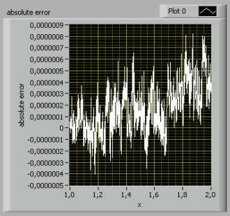
Picture 3: A LabVIEW simulation reveals that the maximum absolute error
may be considered as 8E-7. (mse=2.33)
Compared to the Chebycheff polynomial approximation,
there is a non-negligible loss of accuracy. Another trade-off is the fact that
the number of multiplications depends on the number of significant bits,
whereas the polynomial algorithm keeps the number of operations constant. This
certainly is an issue, if higher precision representations are chosen.
The computational worst case would be to operate a
product with m = b’1111111 11111111 11111111’. This would require 22
multiplications (remember that the last bit may be ignored).
Since the numbers 0 and 1 have the same probability to
appear in m, the average case only requires 11 products.
If we assume the empirical assertion that a
floating-point multiplication needs about 5 times longer than an addition, the
algorithm would be operated within the time of 11*5=55 additions, while the
polynomial approximation would need 9*5+9=50 additions. Thus the average
computing speed may be considered as sensibly equal for both algorithms.
However, a considerable speed gain can be obtained, if
the algorithm is programmed at lowest level, where the access to the
floating-point representation itself is possible. (This is practically required
anyway, since the look-up-table items are selected on the mantissa bits!) One
disadvantage of the polynomial algorithm is the fact that the multiplications
produce un-normalized results that need to be re-expanded and also aligned for
the additions. With the square-root algorithm, such normalizing procedures are
superfluous, since it is guaranteed that after each multiplication the result
is normalized. Thus, calling a primitive floating-point multiplying function
without the normalizing procedure can substantially accelerate the execution.
Another possibility to reduce the computing time may
be given, if less significant mantissa-bits are being considered. Indeed, it
might be useful in some cases to gain speed instead of accuracy. In this case,
the gain, compared to the Chebycheff polynomial approach may be remarkable.
2.4. The influence of the exponent q ¹ 0
Normally mathematicians would consider the exp(x) and
specially the 2x functions differently than presented in this
document, when extending the domain of definition from [1,2[ to
]-¥,+¥[ -or the
portion of this interval that corresponds to the single precision
representation.
In fact they’d prefer writing:
![]()
At first sight, the operation looks like being very
easy and fast, since only the f0 function must be executed and the
result of that operation be multiplied by the rth power of two. The latter
operation could be done simply and rapidly by increasing or decreasing the
binary exponent by |r|. However there is a hook ! The issue is that the
floor-function, representing the truncating of the floating point value, needs
quite an impressive amount of execution steps, because it cannot be deduced by
simple means from the IEEE 754 floating point representation. Therefore we
propose a rather unorthodox approach that will end in a very reduced program
code size.
2.4.1.
First case : q > 0
This
equation doesn’t mean anything else but to compute successive squares of the 21.m
value, each one representing a single multiplying.
2x
rapidly reaches the limit of the IEEE floating point representation as can be
seen in the following series :
q : 1 2 3 4
5 6 7
![]() : 4 16 256 65536
4294967296 1.8446744E19 3.4028236E38
: 4 16 256 65536
4294967296 1.8446744E19 3.4028236E38
For
example: the largest number that can be represented in single precision is
2127 .
1.999999 = 3.4E38. Thus the largest number x that can be computed to
2x is
log2(2128)
=128 Þ q = 7
Example:
Compute y = 29.375
The IEEE
single precision representation of this number gives:
q = 3,
1.m=1.171875
Note that
the relative error grows in a benign way with each multiplication, even if the
2nd condition of the cited theorem in 2.3.1. is no longer fulfilled.
2.4.2.
Second case : q<0
Replacing 2(1.m)
according to formula 1, we get:
![]()
If q = -1,
the equation may be rewritten: ![]()
If q = -2,
it may be written as: ![]()
a.s.o….
To compute
the product for any q, we can operate a simple offset-shift in the look-up
table only depending on the value of q.
Example:
Compute y = 20.146484375
The IEEE
single precision representation of this number gives:
q = -3
and 1.m=1.171875
y = LUT(0+3)
. LUT(3+3) . LUT(5+3) . LUT(6+3)
= 1.0905077 . 1.0108891
. 1.0027112 . 1.0013546
= 1.1068685
Note that "q<-22, 2x will be considered a 1.
2.5. Practical implementation of the algorithm y=2x
Preliminary notes: For this sample the DELPHI language
-former TURBO PASCAL- was chosen because of the better overview concerning
stacked ifs and for loops, than known from C++, even if no such
compiler seems to exist for micro-controllers. The bulk of this section is to
most clearly present an astute and short implementation of the algorithm that
can be easily traduced to any current language. For simplicity, the “NaN”,
“infinity” and “denormalized” handlers have been omitted. However they should
be added to a real implementation in order to keep everything standardized
according to IEEE 754. Obviously the code is set up with respect to the single
precision data representation.
const MAX_ITERATIONS=22; //reduce, if less precision and
more
var LUT: array [0..MAX_ITERATIONS] of
single; //computing speed is
desired
procedure initialize_LUT; //create LUT
var index:integer;
begin //values 0 and MAX_ITERATIONS included in the for
loop!
for index:=0 to MAX_ITERATIONS
do LUT[index]:=power(2,power(2,(-index)));
end;
procedure expand_SGL(x:single;var exponent:integer; var
signum:integer;
var
mantissa:Cardinal); //use var type
to pass data
var tmp:Cardinal; //temporary variable
pIEEE_754_raw: ^Cardinal; //pointer to unsigned 32-bit
variable
begin
pIEEE_754_raw:=@x; //get address of x
if (pIEEE_754_raw^ and
$80000000)=0 then signum:=0 else signum:=1; //0 :+ 1:-
tmp:=pIEEE_754_raw^ and
$7FFFFFFF; //clear sign bit
exponent:=(tmp shr 23)-127; //unbiased exponent
mantissa:=$80000000 or (tmp shl
8); //set hidden bit and shift rest
end;
function two_exp(x:single):single;
var exponent,signum:integer;
mantissa,test:Cardinal;
offset,iterations,index,counter:integer;
temp:single;
begin
expand_SGL(x,exponent,signum,mantissa); //extract data
//special cases
if exponent<-MAX_ITERATIONS then //values below precision
begin
result:=1 //case 2^0.0000... = 1
end else
if exponent=-MAX_ITERATIONS then //no multiplications are needed
begin //since the last item is chosen
only
if signum=0 then
result:=LUT[MAX_ITERATIONS] else
result:=1/LUT[MAX_ITERATIONS]
end else
if exponent>7 then //out of range
begin
if signum=0 then
result:=1E99 else //+infinity
result:=+0 //+0
end else
begin
iterations:=MAX_ITERATIONS; //initialize iterations
//normal cases
if exponent<0 then
begin
offset:=abs(exponent); //get LUT offset
iterations:=iterations+exponent;
//less iterations are required //+= in C++
index:=offset;
//start LUT at offset
temp:=LUT[index] //initialize temporary
variable
end else
begin //exponent>=0
index:=0; //initialize
index
temp:=1 //initialize temp for products
end;
for counter:=1 to
iterations do //now
iterate
begin
index:=index+1; //increment index //+=
operation in C++
mantissa:=mantissa shl 1; //left shift mantissa
test:=mantissa and $80000000; //get most significant bit
//ß
in Assembly language could use faster bit-test
if test<>0 then //check msb
begin
temp:=temp*LUT[index]; //ß
could choose normalized multiplying here //*= in C++
end;
end;
//now do the final multiplying,
if exponent positive
if exponent>=0 then
result:=2*temp else result:=temp; //ß
could fast multiply by 2
//simply increase result’s
//binary
exponent
if signum=1 then
result:=1/result; //negative value,
so inverse
if exponent>0 then
for counter:=1 to exponent
do //now compute squares
result:=result*result; //*= in C++
end;
end;
3.
Study of the calculation of g(x)=ln(x)
3.1.
Simplification to g0(x)=log2(x)
For any
strictly positive real x we have:
![]()
3.2. Study of the function g1(x=1.m) =
log2(1.m)
![]()
Calculating log2(x) may be considered as
the inverse operation to doing 2y with:
x = 2y
Since we have xÎ[1,2[ Þ y=log2(x)
Î [0,1[
and:
![]()
Note: From the IEEE standard point of view, y must be
considered as partly “denormalized”, since the leading 1 must be missing before
the binary point.
Operating the following iterative tests may yield the
set of elements ai:
Example:
Compute y = log2(1.12652145)
Þ m(y) = 001011 Þ y = 0 .
2-1 + 0 . 2-2 + 1 . 2-3
+ 0 . 2-4 + 1 . 2-5 +
1 . 2-6
= 0.125 + 0.03125 + 0.015625
= 0.171875
Instead of using divisions, that need a considerable
computing time, it might be a good idea to additionally use a variant of the
LUT, composed of the inverse values of the initial LUT. This procedure will
allow doing only multiplications. The tests then have the following aspect:
Look-up table with the inverse values:
|
index |
|
|
1 |
0,70710676908493042 |
|
2 |
0,840896427631278174 |
|
3 |
0,917004048824310303 |
|
4 |
0,957603275775909424 |
|
5 |
0,978572070598602295 |
|
Etc. |
|
3.3. Note for the practical implementation of the
algorithm y=log2(x)
Since the successive values of x and the LUT numbers
that are used with the comparisons are always normalized, the comparisons can be
fast computed. But this time the multiplications are operated with
un-normalized numbers (2nd LUT). However, it is obvious that the
multiplications always remain in the interval ]0,1[. A low level fast
multiplying routine can be set up for these numbers, increasing the computing
speed. Nonetheless the log2 algorithm implementation seems trivial
and a sample code can be omitted in this document.
![]()
Conclusion
This algorithm package may be helpful to implement
fast calculations for the exp(x) and the ln(x) functions in the special case
of IEEE 754 standard single precision
representation to any desired precision in the given range.