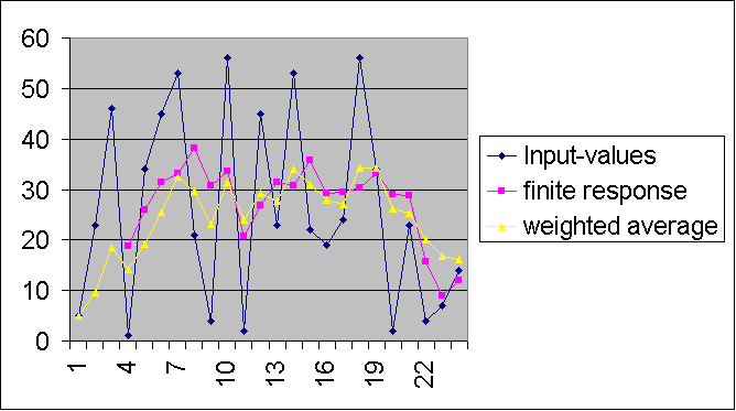
In the very interesting book Extreme Mindstorms one of the authors Dave Baum explains the concept of the finite response. The idea is to calculate the average of let's say the N = 4 last light- sensor-values. The RCX 2.0 firmware allows arrays, so Dave uses N array-fields to store the most recent input-values. Everytime a new value appears, the oldest of the N values is replaced.
For example: (The most recent value is marked with white colour)
| one | two | three | four | average |
| 5 | 23 | 46 | 1 | 19 |
| 34 | 23 | 46 | 1 | 26 |
| 34 | 45 | 46 | 1 | 32 |
| 34 | 45 | 53 | 1 | 33 |
| 34 | 45 | 53 | 21 | 38 |
| 4 | 45 | 53 | 21 | 31 |
| 4 | 56 | 53 | 21 | 34 |
The utility of such a procedure is clear. Many times you have to observe light, compass or other inputs. Often it appears that instant sensor-values are below or above a limit-value you use for decision taking. They may even swing around a certain value. This makes adequat robot response quite difficult. The solution is to take average-values instead of momentous. This trick is comparable to the use of a capacitor in electronics. The system avoids peak-values because of a certain inertial effect.
Unfortunately, in a limited environment like the RCX, specially if you don't dispose of the 2.0 firmware (this is the case, when you work with Robolab), Dave's proposal is not the best solution.
Infinite response
We use a much simpler procedure called infinite response to get a very similar result. The trick is always to calculate the ponderous average or weighted average:
x' = (a * x + b * r) / (a + b)
where x is the last average, x' the new average, r the most recent input-value, a and b are coefficients which define the weight of the old average and the new reading. A given input value has a limited on the result forever.
In the example above:
x' = (3 * x + r ) / 4
| last average | input value | new average |
| 19 | 1 | 14 |
| 14 | 34 | 19 |
| 19 | 45 | 26 |
| 26 | 53 | 32 |
| 32 | 21 | 30 |
| 30 | 4 | 23 |
| 31 | 56 | 31 |
As you can see the result is nearly the same as for the finite response.
| Dave writes:
" Most applications use infinite response because, as you demonstrated, it is a simpler algorithm, requires less storage, and has nearly the same effect as finite response in many typical situations. In fact, I'd probably use infinite response myself most of the time on the RCX, but for the book I wanted an example that used the arrays, so I chose finite response. One area infinite response can get you into trouble is if your input source has occasional spikes of noise, but you also want to detect pulses. For example, let's say a typical series of readings looks like this ... 2, 3, 2, 2, 3, 2, 3, 200, 2, 3, 2, 3, 2, 2, 3, 2, 3, 100, 101, 100, 101, 100, 2, 3, 3, ... and you want to reject that noise sample of 200, but detect the pulse around 100. With finite response, making N greater than 1 and less than the minimum pulse (lets say 4) would ensure detection of the pulse while rejecting noise. With infinite response it can be very difficult to set appropriate weights. Emphasis of the new sample will cause noise to have adverse effects, while emphasis of the old average will make it difficult to detect short pulses. Basically, finite response gives you a sharper cut-off. If the decision is a boolean one, then infinite response can be used along with moving th threshold values in a bit to account for the fact that a short pulse won't raise the average all the way to the pulse value. However, for analog applications (let's say some sort of peak detection with noise rejection), there aren't any thresholds to move. " Thanks Dave for these explanations! |